In A Short Pedagogical Note, Nassim Taleb outlines his specific objection to Extreme Value Theory (EVT), imploring us to forget about it (fuhgetaboudit!). Unfortunately, financial panics and hundred-year floods continue to remind us of EVT, as do pandemics. Juxtaposing A Short Pedagogical Note with Taleb’s treatise, Tail Risk of Contagious Diseases, one might conclude that the risk engineer occupies the ultimate hedged position as a both an opponent and proponent of EVT.
Evidently, Taleb endorses the use of EVT as an alternative to the “naive interpolations and expected averages for risk management purposes.” The apparent contradiction between his recent writings could be resolved as his railing against the misuse, not the use, of statistical machinery. In an effort to better understand the basics of EVT, this post reverse-engineers A Short Pedagogical Note. Since we don’t have access to the software that Taleb used, we supplement Taleb’s examples with illustrative software snippets and figures of our own. Those figures are then sanity-checked against Taleb’s.
We begin with $ E_j $, the maximum of a single normally distributed sample with N data points:
$$ E_j = Max\{ Z_{i,j} \}^N_{i = 1} $$
Then, we take the maximum of that normal sample, and repeat the sampling process $M$ times. The resulting set $E$ contains $M$ points, the maxima of $M$ samples of size $N$:
$$ E_j = \{ Max\{ Z_{i,j} \}^N_{i = 1}\}^M_{j=1} $$
If $Z$ refers to a standard normal distribution, the result is the Gumbel distribution:
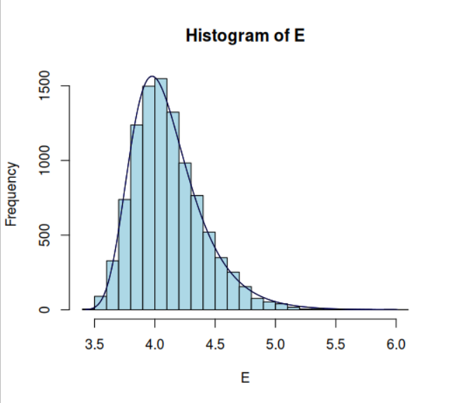
The following code will reproduce the Gumbel Distribution:
library(fitdistrplus)
library(extRemes)
library(evd)

### Case 1: Gumbel
E <- list()
for(i in 1:10^4){ E[[i]] = max(rnorm(3*10^4, mean = 0, sd = 1)); print(i)}
E <- do.call(rbind, E)
E <- as.numeric(E)
h <- hist(E, breaks = 30, ylim = c(0, 1800), col = "#0CB1B9")
params <- fitdist(E, "gumbel", method = "mse", lower = c(0, 0, 0), start = list(loc=0.45, scale=36), keepdata = T)
xfit <- seq(min(E), max(E), length = 500)
yfit <- dgumbel(xfit, loc = params$estimate[[1]], scale = params$estimate[[2]])
yfit <- yfit * diff(h$mids[1:2])*length(E)
lines(xfit, yfit, col="blue", lwd=2)
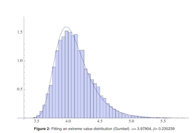
Here is the Gumbel distribution from the pedagogical paper:
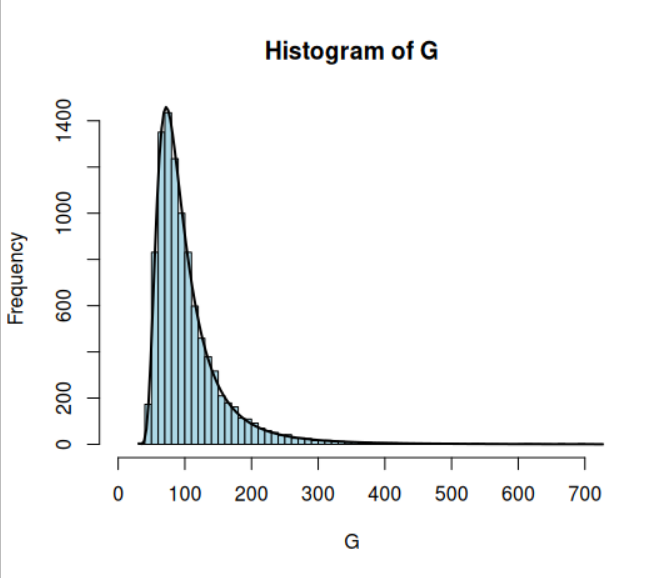
If, however, we begin with a heavy tail (Student’s T-distribution with three degrees of freedom), and proceed exactly as before, we get a Fréchet distribution:
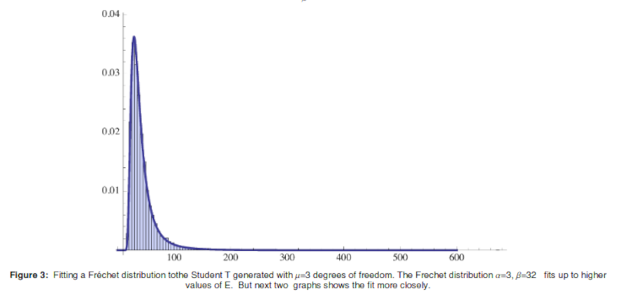
Here is the Fréchet distribution from the pedagogical paper:
The following code will reproduce the Fréchet distribution.
### Case 2: Fréchet
G <- list()
for(i in 1:10^4){ G[[i]] = max(rt(10^3, df = 3, ncp = 3)); print(i)}
G <- do.call(rbind, G)
G <- as.numeric(G)
h <- hist(G, breaks = 300, ylim = c(0, 1800), xlim = c(0, 600), col = "#0CB1B9")
params <- fitdist(G, "frechet", method = "mse", lower = c(0, 0, 0), start = list(loc=0.45, scale=36, shape=3), keepdata = T)
xfit <- seq(min(G), max(G), length = 500)
yfit <- dfrechet(xfit, loc = params$estimate[[1]], scale = params$estimate[[2]], shape = params$estimate[[3]])
yfit <- yfit * diff(h$mids[1:2]) * length(G)
lines(xfit, yfit, col="blue", lwd=2)
The final tables illustrate the problem of parameter estimation:
### Create the final chart
loc1 = params$estimate[[1]]
scale1 = params$estimate[[2]] # Beta in Taleb's paper
shape1 = params$estimate[[3]]
shape1

shape1

alphas = seq(1,5, by = 0.25)

three_beta = list()

ten_beta = list()
twenty_beta = list()

for(i in 1:length(alphas)){
  three_beta[[i]] = integrate(dfrechet, lower = 3 * scale1, upper = Inf, loc = loc1, scale = scale1, shape = alphas[[i]])$value ### Scale is the exponent
  ten_beta[[i]] = integrate(dfrechet, lower = 10 * scale1, upper = Inf, loc = loc1, scale = scale1, shape = alphas[[i]])$value ### Scale is the exponent
  twenty_beta[[i]] = integrate(dfrechet, lower = 20 * scale1, upper = Inf, loc = loc1, scale = scale1, shape = alphas[[i]])$value ### Scale is the exponent
  print(i)
}

three_beta = do.call(rbind, three_beta)
ten_beta = do.call(rbind, ten_beta)
twenty_beta = do.call(rbind, twenty_beta)

three_beta_inv = 1 / three_beta
ten_beta_inv = 1 / ten_beta
twenty_beta_inv = 1/ twenty_beta

final_chart = cbind.data.frame(alphas, three_beta_inv, ten_beta_inv, twenty_beta_inv)
final_chart
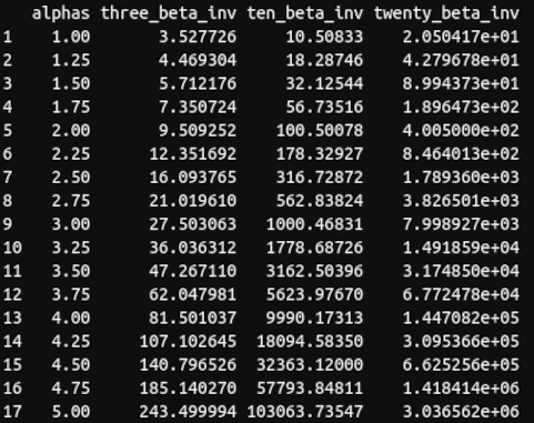
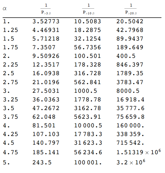
Taleb’s conclusion is as follows:
Consider that the error in estimating the $\alpha$ distribution is quite large, often > 1/2, and typically overstimated [sic]. So we can see that we get the probabilities mixed up > an order of magnitude. In other words the imprecision in the computation of the $\alpha$ compounds in the evaluation of the probabilities of extreme values.
Since this conclusion follows from Taleb’s practical experience, which is substantial, we accept it at face value. It stands to reason that the parameters governing the precise shapes of heavy-tail distributions are in fact difficult to estimate.
The lopsided dangers posed by the hypertrophy of a scorpion’s claws versus its sting inspired the Roman aphorism “in cauda venenum”. Literally translated as poison in the tail, it is a metaphoric warning about hidden danger and the spectacles that distract us from it. An engineering civilization like Rome that survived urbanization, pandemic, civil war, and currency debasement would have marveled at the quantification of risk using computational tools—and at modern parallels.