In a prior blog post, Is it Normal?, we began with two normal distributions and summed their frequencies to obtain a Gaussian mixture. In this post, we begin with a Gaussian mixture and deploy the Expectation-Maximization (EM) algorithm to decompose a given Gaussian mixture into its component distributions. Example code is included, and the results of these examples are contrasted with that of an R package mixtools, a professional software release which is based upon based upon work supported by the National Science Foundation under Grant No.ES-0518772. (3)
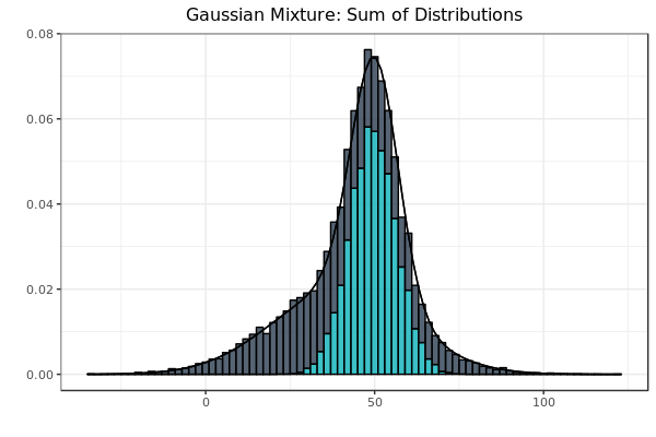 Fig. 1: The summation of frequencies is represented by stacked bars. As before, the black line at the perimeter of the figure is the idealized equation of the actual sample that it bounds.
If the graph in Fig. 1 represented credit card transactions, all transactions would be either legitimate or fraudulent, and nothing in between. Classifying the transactions as such would therefore partition the sample space as the sets would be mutually disjoint. However, there would be a large class imbalance between the legitimate and fraudulent transactions, as the overwhelming majority of credit card transactions are legitimate. In Fig. 1, the class sizes were equal so as to serve as a visual aid. Strategies designed to deal with the class imbalances of credit-card transactions will be the subject of following posts.
The above figure can be produced using the following code:
### Algorithm 8.1 Implementation
options(digits = 15)
### Prerequisite code from our previous post, "Is It Normal"
# Make sure to install.packages("pacman") if it isn't already available
pacman::p_load("ggplot2", # pacman::p_load is an awesome 2-for-1 substitute for base R install.packages() and library()
               "RColorBrewer",
               "extrafont",
               "gridExtra") # With pacman, you can avoid errors due to library discrepancies between environments!

### custom function returning dnorm equivalent of Gaussian Mixture
gaussian_mixture <- function(x, mean1, mean2, sd1, sd2){
  coeff1 = 1/sqrt(2*pi * sd1^2)
  coeff2 = 1/sqrt(2*pi * sd2^2)
  freq = coeff1 * exp( -((x - mean1)^2) / (2*sd1^2)) + coeff2 * exp(-(x - mean2)^2 / (2*sd2^2))
  return(freq)
}

### Define standard-normal random variables
set.seed(7654) # keep this seed
sample_size = 10^4
dist1 = rnorm(10^4, 40, 20) # 40:20 (mean-sd)
dist2 = rnorm(10^4, 50, 7)  # 50:7 (mean-sd)
df1 <- data.frame(flip = factor(rep(c("H", "T"), each = sample_size)), value = round(c(dist1, dist2))) # data set under consideration

### Add the distributions as opposed to adding the random variables
gauss_mix <- ggplot(df1, aes(x = value, color = flip, fill = flip)) +
  geom_histogram(aes(y = ..density..), position = "stack", alpha = 0.8, binwidth = 2) +
  scale_color_manual(values = c("#000000", "#000000", "#999999")) +
  scale_fill_manual(values = c("#2C3E50", "#0CB1B9", "#000000")) +
  labs(title = "Gaussian Mixture: Sum of Distributions", x = "", y = "") +
  theme_bw() +
  theme(plot.title = element_text(hjust = 0.5)) +
  theme(legend.position = "none") +
  theme(text = element_text(size = 10, family = "Montserrat")) +
  stat_function(fun = gaussian_mixture, args = list(mean1 = mean(dist1),
                                                    sd1 = sd(dist1),
                                                    mean2 = mean(dist2),
                                                    sd2 = sd(dist2)))
gauss_mix
The following algorithm is abstracted from the Elements of Statistical Learning. (1):
Algorithm 8.1: Expectation-Maximization (EM) Algorithm for Two-Component Gaussian Mixture
- Take initial guesses for the parameters: $$\hat{\mu}_1, \hat{\sigma}_1, \hat{\mu}_2, \hat{\sigma}_2, \hat{\pi}.$$
- Expectation Step. Compute the responsibilities: $$ \hat{\gamma}_i = {\pi \phi_\hat{\theta_2}(y_i) \over (1-\hat{\pi})\phi_\hat{\theta_1}(y_i) + \phi_\hat{\theta_2}(y_i)}, \ i = 1, 2, …,N. $$
- Maximization Step. Compute the weighted means and variances: $$ \hat{\mu}_1 = {\sum_{i=1}^N (1-\hat{\gamma}_i) y_i \over \sum_{i=1}^N (1-\hat{\gamma}_i)}, \ \hat{\sigma}^2_1 = {\sum_{i=1}^N (1-\hat{\gamma}_i)(y_i - \hat{\mu}_1)^2 \over \sum_{i=1}^N (1-\hat{\gamma}_i)} $$ $$ \hat{\mu}_2 = {\sum_{i=1}^N \hat{\gamma}_i y_i \over \sum_{i=1}^N \hat{\gamma}_i}, \ \hat{\sigma}^2_2 = {\sum_{i=1}^N \hat{\gamma}_i(y_i - \hat{\mu}_1)^2 \over \sum_{i=1}^N \hat{\gamma}_i} $$ and the mixing probability: $$\hat{\pi} = {\sum_{i=1}^N \hat{\gamma}_i \over N}.$$
- Iterate steps 2 and 3 until convergence.
To start, both $\hat{\mu}_1$ and $\hat{\mu}_2$ were established through random selection of a values from the distribution. (1) Both $\hat{\sigma}_1,\ \hat{\sigma}_2 $ were set to the standard deviation of the overall distribution (the algorithm, as written, refers to the variance, which is the square of standard deviation). (1)
The formula, $\hat{\pi} = {\sum_{i=1}^N \hat{\gamma}_i \over N}$, is the maximum likelihood estimation for the proportion of observations coming from class 2 for each iteration of the EM algorithm. (1) The EM algorithm is a two-step process. (2) Whereas the expectation step calculates maximum likelihood estimation of observed data and parameters, the maximization step uses conditionally expected values in lieu of unobserved parameters. (2)
The above algorithm is implemented in the following code:
### Step 1: Take initial guesses
data = df1$value # look at distribution without head/tails breakdown

EM = function(data){
  set.seed(1234) # make function idempotent
  inital_mean_index = sample(1:length(data), 2)
  mean1 = data[inital_mean_index[[1]]]
  mean2 = data[inital_mean_index[[2]]]
  mean1
  mean2
  pi_hat = 0.5 # the mixing probability
  sd1 = sd(data)
  sd2 = sd(data)

  mean1_list = list()
  mean2_list = list()
  sd1_list = list()
  sd2_list = list()

  # Step 2: Expectation step
  rep = 1
  repeat{
    coeff1 = 1/sqrt(2*pi * sd1^2)
    coeff2 = 1/sqrt(2*pi * sd2^2)
    freq1 = function(x) coeff1 * exp(-((x - mean1)^2 ) / (2*sd1^2))
    freq2 = function(x) coeff2 * exp(-(x - mean2)^2 / (2*sd2^2))
    freq1(mean1)
    freq2(mean2)
    gamma_hat = (pi_hat * freq2(data) / ( (1 - pi_hat) * freq1(data) + pi_hat * freq2(data) ))

    ### Step 3: Maximization step
    mean_hat_1 = sum((1 - gamma_hat)*data)/sum(1-gamma_hat)
    mean_hat_2 = sum((gamma_hat)*data)/sum(gamma_hat)
    sd_hat_1 = sqrt(sum((1 - gamma_hat)*((data - mean1)^2))/sum(1-gamma_hat))
    sd_hat_2 =  sqrt(sum((gamma_hat)*((data - mean2)^2))/sum(gamma_hat))
    pi_hat = mean(gamma_hat)

    ### reset parameters and prepare to repeat
    mean1 = mean_hat_1
    mean2 = mean_hat_2
    sd1 = sd_hat_1
    sd2 = sd_hat_2

    ### monitor convergence
    mean1_list[[rep]] = mean1
    mean2_list[[rep]] = mean2
    sd1_list[[rep]] = sd1
    sd2_list[[rep]] = sd2

    error = 10^-8
    if(rep > 1 &&
       rep <= 1000 && # cap for repetitions in case of non-convergence
       abs(mean1_list[[rep]] - mean1_list[[rep-1]]) < error &&
       abs(mean2_list[[rep]] - mean2_list[[rep-1]]) < error &&
       abs(sd1_list[[rep]] - sd1_list[[rep-1]]) < error &&
       abs(sd2_list[[rep]] - sd2_list[[rep-1]]) < error)
    {
      break
    }
    rep = rep + 1
  }
  ### Monitor convergence
  mean1_list = do.call(rbind, mean1_list)
  mean2_list = do.call(rbind, mean2_list)
  sd1_list = do.call(rbind, sd1_list)
  sd2_list = do.call(rbind, sd2_list)
  parameters = cbind.data.frame(mean1_list, mean2_list, sd1_list, sd2_list)

  return(list(mean1_list, mean2_list, sd1_list, sd2_list, parameters))
}

variables = EM(data)
The EM function returns stepwise parameter convergence illustrated by the following graph:
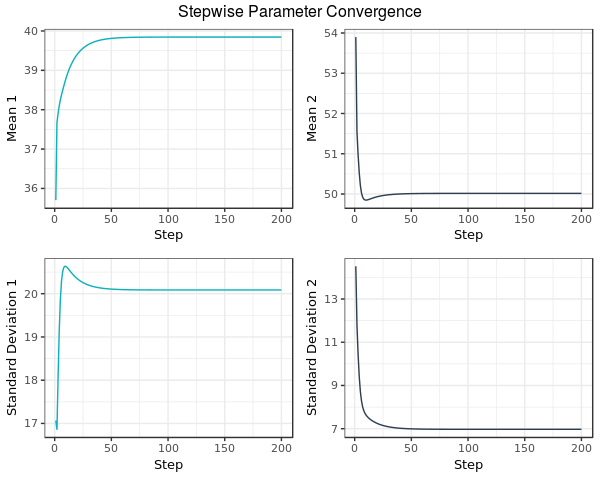 Fig. 2: In this example, the process is halted once all parameters move less that $10^{-8}$ per iteration, or after 1000 iterations, whichever condition is met first. At this step, the EM algorithm terminates and the estimates for both means and standard deviations are returned by the EM function in the aforementioned code.
The Stepwise Parameter Convergence graph was created by the following code:
### Visualize the convergence of all parameters
param_mix1 <- ggplot(variables[[5]], aes(x = c(1:length(variables[[1]])))) +
  geom_line(stat = "identity", aes(y = variables[[1]]), col = "#0CB1B9") +
  theme_bw() +
  theme(plot.title = element_text(hjust = 0.5)) +
  theme(legend.position = "none") +
  theme(text = element_text(size = 10, family = "Montserrat")) +
  ylab("Mean 1") +
  xlab("Step")

param_mix2 <- ggplot(variables[[5]], aes(x = c(1:length(variables[[2]])))) +
  geom_line(stat = "identity", aes(y = variables[[2]]), col = "#2C3E50") +
  theme_bw() +
  theme(plot.title = element_text(hjust = 0.5)) +
  theme(legend.position = "none") +
  theme(text = element_text(size = 10, family = "Montserrat")) +
  ylab("Mean 2") +
  xlab("Step")

param_mix3 <- ggplot(variables[[5]], aes(x = c(1:length(variables[[3]])))) +
  geom_line(stat = "identity", aes(y = variables[[3]]), col = "#0CB1B9") +
  theme_bw() +
  theme(plot.title = element_text(hjust = 0.5)) +
  theme(legend.position = "none") +
  theme(text = element_text(size = 10, family = "Montserrat")) +
  ylab("Standard Deviation 1") +
  xlab("Step")

param_mix4 <- ggplot(variables[[5]], aes(x = c(1:length(variables[[4]])))) +
  geom_line(stat = "identity", aes(y = variables[[4]]), col = "#2C3E50") +
  theme_bw() +
  theme(plot.title = element_text(hjust = 0.5)) +
  theme(legend.position = "none") +
  theme(text = element_text(size = 10, family = "Montserrat")) +
  ylab("Standard Deviation 2") +
  xlab("Step")

grid.arrange(param_mix1, param_mix2, param_mix3, param_mix4, ncol = 2, top = "Stepwise Parameter Convergence")
The performance of normalmixEM function from the mixtools package can be contrasted with that of the EM function offered in this blog post with the following code, both in terms of performance and numerical result:
### Compare the competition: mixtools
pacman::p_load("mixtools",
               "microbenchmark") # pacman is your friend, for simple and reliable portability.
variables = EM(data)
mean1 = as.numeric(tail(variables[[1]], 1))
mean2 = as.numeric(tail(variables[[2]], 1))
sd1 = as.numeric(tail(variables[[3]], 1))
sd2 = as.numeric(tail(variables[[4]], 1))
competition = normalmixEM(data, ECM = F)
### Disclaimer: microbenchmark iterates many times and these example distributions are relatively large; running this benchmark is disabled by default for brevity.
# microbenchmark(normalmixEM(data, ECM = F))
# microbenchmark(EM(data))
round(sort(competition$sigma) - sort(c(sd1, sd2)), 5)
round(sort(competition$mu) - sort(c(mean1, mean2)), 5)
The normalmixEM function from the mixtools package took approximately 267 milliseconds to converge whereas the EM function of this blog post took approximately 247 milliseconds. The functions were run on a single thread of a stock Ryzen 1700X (3.6 GHz base clock). These values are the medians as reported by the microbenchmark function. The differences in output between the EM function written in the blog post and that of the mixtools package are all equal to or less than five in 100,000.
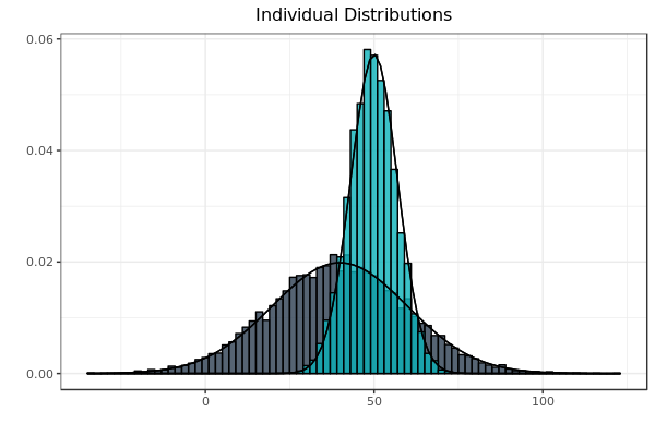 Fig. 3: Distributions reflect the parameters computed by the author’s implementation of the EM algorithm on the data set which produced Fig. 1. As before, each sample is bounded by its idealized curve.
Fig. 3 can be produced with the following code:
### Superimposed equations use parameters computed by EM Algorithm
df1 <- data.frame(flip = factor(rep(c("H", "T"), each = sample_size)), value = round(c(dist1, dist2)))

ind_dist <- ggplot(df1, aes(x = value, color = flip, fill = flip)) +
  geom_histogram(aes(y = ..density..), position = "identity", alpha = 0.8, binwidth = 2) +
  scale_color_manual(values = c("#000000", "#000000", "#999999")) +
  scale_fill_manual(values = c("#2C3E50", "#0CB1B9", "#000000")) +
  labs(title = "Individual Distributions", x = "", y = "") +
  theme_bw() +
  theme(plot.title = element_text(hjust = 0.5)) +
  theme(text=element_text(size = 10, family="Montserrat")) +
  theme(legend.position = "none") +
  stat_function(fun = dnorm, args = list(mean = mean1, sd = sd1)) +
  stat_function(fun = dnorm, args = list(mean = mean2, sd = sd2))

ind_dist
Conclusion
The EM algorithm is a form of unsupervised learning as no response variable is present. It excels at modeling the parameters of the probability density functions of the given input. Neither convergence nor a globally optimal result is guaranteed. Gaussian mixtures—and the EM algorithm which abstracts the underlying distribution—see diverse application in genomics, risk management and the detection of credit card fraud. These topics will be the subject of future blog posts.
Works Cited
(1) Hastie, Trevor, et al. The Elements of Statistical Learning: Data Mining, Inference, and Prediction. Springer, 2013.
(2) Hilbe, Joseph M., and Andrew P. Robinson. Methods of Statistical Model Estimation. CRC Press, 2013.
(3) Tatiana Benaglia, Didier Chauveau, David R. Hunter, Derek Young (2009). mixtools: An R Package for Analyzing Finite Mixture Models. Journal of Statistical Software, 32(6), 1-29. URL http://www.jstatsoft.org/v32/i06/.
Packages Used
Baptiste Auguie (2017). gridExtra: Miscellaneous Functions for “Grid” Graphics. R package version 2.3.https://CRAN.R-project.org/package=gridExtra
Erich Neuwirth (2014). RColorBrewer: ColorBrewer Palettes. R package version 1.1-2.https://CRAN.R-project.org/package=RColorBrewer
H. Wickham. ggplot2: Elegant Graphics for Data Analysis. Springer-Verlag New York, 2016.
Olaf Mersmann (2018). microbenchmark: Accurate Timing Functions. R package version 1.4-6.https://CRAN.R-project.org/package=microbenchmark
Rinker, T. W. & Kurkiewicz, D. (2017). pacman: Package Management for R. version 0.5.0. Buffalo, New York. http://github.com/trinker/pacman
Tatiana Benaglia, Didier Chauveau, David R. Hunter, Derek Young (2009). mixtools: An R Package for Analyzing Finite Mixture Models. Journal of Statistical Software, 32(6), 1-29. URL http://www.jstatsoft.org/v32/i06/.
Winston Chang, (2014). extrafont: Tools for using fonts. R package version 0.17. https://CRAN.R-project.org/package=extrafont