Solubility can be defined as the propensity of a solid, liquid, or gaseous quantity (solute) to dissolve in another substance (solvent). Among many factors, temperature, pH, and pressure, and entropy of mixing all impact solubility. (Loudon, Parise 2016) Solvents can be classified as either protic or aprotic, polar or apolar, and donor or nondonor. (Loudon, Parise 2016) The specifics, illustrated by the solubility data set from Applied Predictive Modeling, are beyond the scope of this paper. The most important rule for understanding solubility is “like dissolves like.” (Loudon, Parise 2016) In other words, polar solvents, like water, dissolve polar compounds such as ethanol easily, whereas nonpolar compounds, such as olive oil, hardly dissolve in water, forming a heterogeneous mixture instead.
Characteristics of the solubility Data Set
This paper follows the solubility data set in Applied Predictive Modeling, builds on the included code samples, and depicts three different predictive models for solubility as a function of 228 available predictors. Each column of the solubility dataset corresponds to a predictor.
An excerpt of the solubility data set appears below.
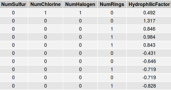
Note that all of the variables displayed in this table are quantitative. The numbers of sulfurs, chlorines, halogens, and rings are all integer values whereas variables such as Hydrophilic Factor, are continuous. The solubility data set was divided into both a test set and a training set. The training set is approximately three times larger than the testing set.
Next, we have a look at the response variable.
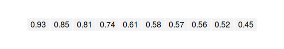
The first 10 of 316 values of the test set for solubility appear above. These values are the logarithms of compound solubility.
Solubility Plots
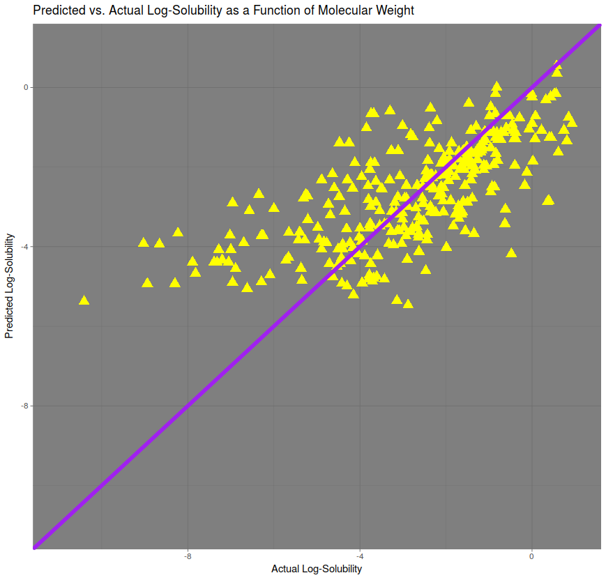
The heaviest predictor of solubility, in terms of correlation, was molecular weight. A linear model was created in order to predict solubility, and predictions for the test set were plotted against the actual values in the figure above. The line of perfect prediction, in purple, implies a correlation of 1. The correlation here is approximately 75%. The root mean squared error (RMSE), is approximately 1.51.
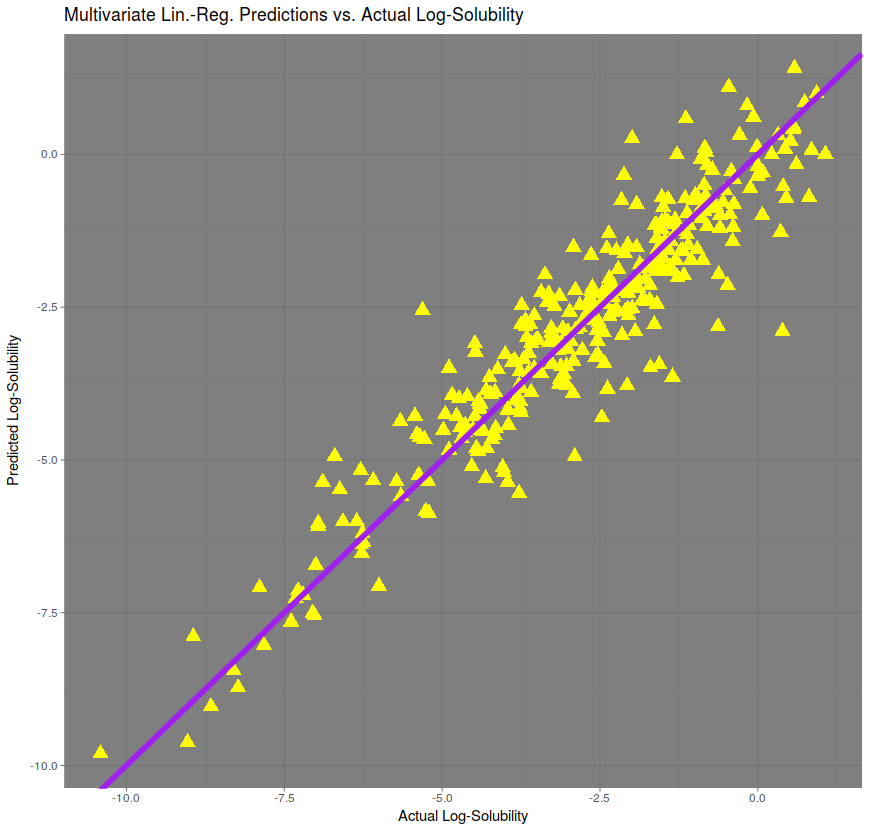
A multivariate prediction, automatically fitted by the R Programming Language, gives a much better prediction, with a correlation of approximately 95%. The RMSE is approximately 0.746, performing roughly twice as well as the regression on molecular weight only.
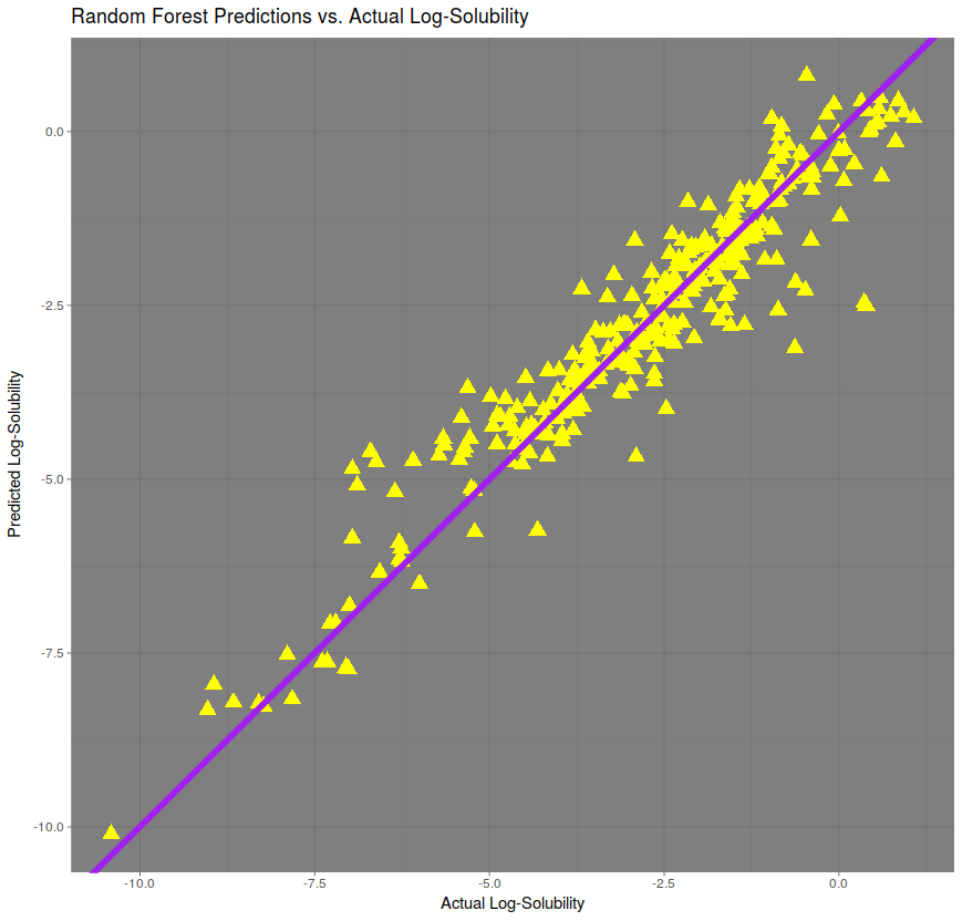
Best of all is the random forest regression, with a correlation of over 95% and an RMSE of only 0.65. The R code used to generate this random forest model used only the randomForest function from package of the same name, with importance = TRUE and ntrees = 1000.
Conclusion
Random forest regression can outperform multivariate regression and seems well suited to large data sets with many predictors. However, random forests for regression applications can be computationally intensive and require that the practitioner select both tuning parameters as well as the number of trees for the forest. (Kuhn, Johnson 2016) Future posts will delve deeper into the specifics of random forests regression.
Works Cited
Kuhn, M., & Johnson, K. (2016). Applied Predictive Modeling. New York: Springer.
Loudon, G. M., & Parise, J. (2016). Organic Chemistry. New York: W.H. Freeman, Macmillan Learning.