The Curse of Dimensionality refers to the phenomenon by which all observations become extrema as the number of free parameters, also called dimensions, grows. In other words, hyper-dimensional cubes are almost all corners. Corners, in this context, refer to the volume contained in cubes outside of the volume contained by inscribed spheres regardless of dimension. The Curse of Dimensionality is of central importance to machine learning datasets which are often high dimensional. (Hastie, Tibshirani and Friedman, 2013) For techniques that rely on local approaches, such as the K-Nearest Neighbors algorithm, it is overwhelmingly likely that a small number of data points scattered in high-dimensional space will fail to conform to the boundaries of any local neighborhood. (James 2017) Moreover, in high-dimensional settings, the multicollinearity problem by which just about any variable in the model can be written as a linear combination of the others, makes it very difficult to determine which variables should be included in linear regression. (James 2017) This post seeks to build understanding of the Curse of Dimensionality through analogy to the familiar, lower-dimensional shapes of circles, squares, spheres, and cubes.
We begin with the lower dimensions and build our case sequentially by adding dimensions. Consider a 2-sphere, more commonly known as a circle. Ratios of volumes will be determined by the throwing of probabilistic “darts” at the unit square, the square that occupies (-1,1) x (-1,1). The points inside the unit circle are defined by the inequality $x_1^2 + x_2^2 \leq 1$. The ratio of unit-circle area to unit-square area can be computed analytically using the familiar $\pi r^2$ formula for the former and the formula $(2r)^2 = 4 r^2$ for the latter.
This ratio of unit circle to unit square area will then be $\pi r^2 / 4 r^2 = \pi / 4$, which is approximately 78.53%. The “throwing” of 100,000,000 “darts” was simulated by drawing 100,000,0000 $x_1$ values from the uniform distribution, U(-1,1), and also drawing the same number of $x_2$ values from the same. In contrast to the analytical method of finding the volumes of solids, using formulas, this method of calculating volumes is probabilistic, where the ratio of “hits” to the number of darts thrown will reveal volume to an arbitrary degree of precision.
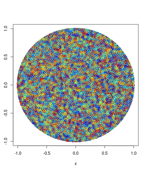
This circular plot could also be called a 2-sphere, a two-dimensional sphere. Coordinates for the x_1 and x_2 axis were drawn randomly from a uniform distribution with bounds (-1,1). Points satisfying the inequality $x_1^2 + x_2^2 \leq 1$ fill the circle. Points satisfying $x_1^2 + x_2^2 > 1$ were not graphed, and are represented by white space. Approximately 78% of the unit square spanning (-1,1) x (-1,1) is accounted for by the area of the circle.
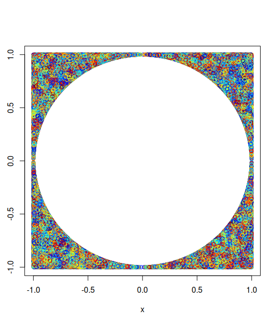
This plot is the perfect complement of the prior one; points satisfying $x^2 + y^2 > 1$ are indicated by the multi-colored links. The colored portion in this figure accounts for only about 22% of the unit square’s area. Next, we move on the three-dimensional analogue of a circle inscribed in a square, a sphere inscribed in a cube.
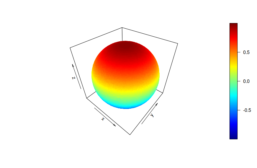
Here we have a unit sphere sitting inside of a unit cube. Each edge of the cube has length 2; the radius of the sphere is one. You may recall the volume of a sphere obeys the following formulas, $4 \pi r^3 / 3$. The volume of the cube is of course, $2^3 = 8$. Taking the ratio of the sphere’s volume evaluated at r = 1 to that of the cube yields $4 \pi / 24 = \pi / 6$, which is just over 52%. This means that approximately 48% of the unit cube’s volume lies outside the sphere, in the corners. The percentage of area covered by the unit square was 78%; the percentage of volume occupied by the unit sphere was only 52%. Where does this trend lead?
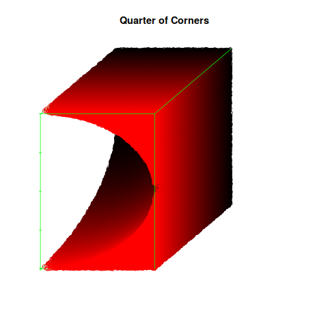
Here is one of four symmetric quadrants where the volume outside of the sphere is shaded in red and black. The sphere itself is missing from this diagram. The ratio of the missing volume to the shaded volume will be as before, approximately 52%.
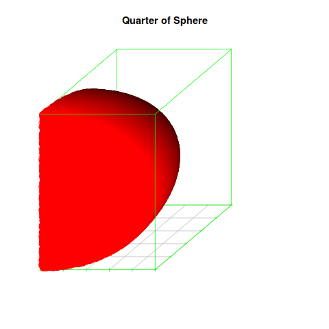
This is the perfect complement to the above figure, a quadrant of the unit sphere. The ratio of shaded volume to missing volume will be as before, approximately 52%.
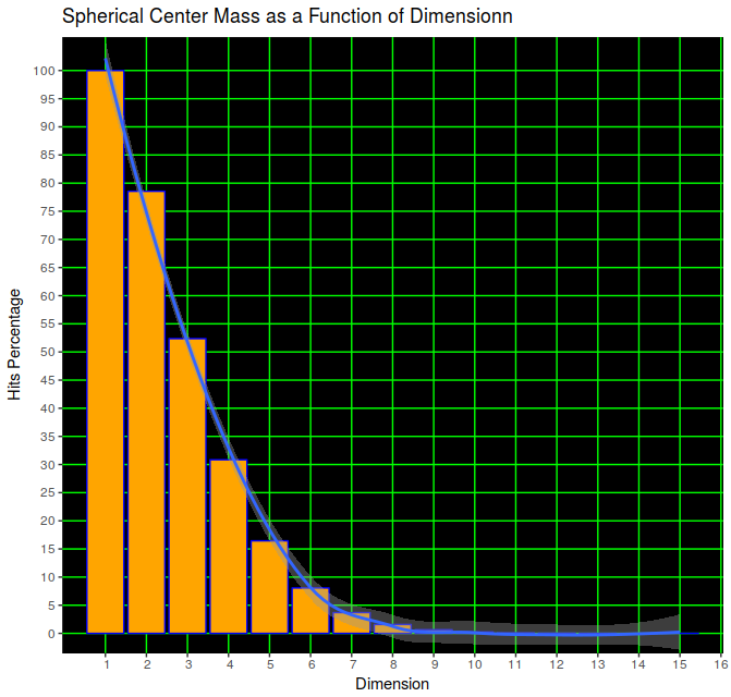
The percentage of center mass, defined as the ratio of an inscribed hypersphere’s volume to the volume of its containing hypercube falls exponentially with increasing dimension. The figure begins with the degenerate case of a one-dimensional circle, also known as a line. Unsurprisingly, 100% of the points drawn from a uniform distribution from the interval (-1,1) will lie on in the interval (-1,1). By the time the number of dimensions equals four, the inscribed 4-sphere accounts for only about 30% of the 4-cube’s total volume. As the number of dimensions increases, the hypersphere’s share of total volume continues approaches zero asymptotically.
Conclusion
This post has approached the Curse of Dimensionality from a brute-force probabilistic perspective. An intuitive alternative explanation for the Curse of Dimensionality is offered. For an n-tuple, $(x_1, x_2, …, x_n)$, only one of the $x_i$ has to be close to 1 in order to make the entire n-tuple an extreme value. As n increases, the probability that a randomly selected n-tuple will also be an extreme value increases dramatically because the n-tuple has n opportunities to hold at least one or more extreme values. If only value of an n-tuple is extreme, the entire n-tuple becomes an extremum, as the one extreme value lifts the volume element out of the local sphere and into the corners.
To an extent, the Curse of Dimensionality can be mitigated by datasets whose coordinates each have a very high degree of central tendency. If each $x_i$ was drawn from the normal distribution with a small, fractional standard deviation, higher-dimensional spheres would be slightly favored in terms of the number of points they contain relative to their surroundings. But even in these cases, the Curse of Dimensionality can be postponed but never entirely avoided. The exponential growth of points as a function of dimension will always overwhelm probability distributions with even the highest degree of central tendency.
Strategies for addressing the Curse of Dimensionality in a machine-learning context will be a topic of future posts.
Works Cited
James, Gareth, et al. (2017). An Introduction to Statistical Learning: with Applications in R. Springer.
Hastie, T., Tibshirani, R. and Friedman, J. (2013). The elements of statistical learning. 7th ed. In text: (Hastie, Tibshirani and Friedman, 2013)
Packages Used
Karline Soetaert (2017). plot3D: Plotting Multi-Dimensional Data. R package version 1.1.1. https://CRAN.R-project.org/package=plot3D
Ligges, U. and Mächler, M. (2003). Scatterplot3d - an R Package for Visualizing Multivariate Data. Journal of Statistical Software 8(11), 1-20.
R Core Team (2017). R: A language and environment for statistical computing. R Foundation for Statistical Computing, Vienna, Austria. URL https://www.R-project.org/.
